Clustering
Overview
Introduction Clustering is an unsupervised learning approach that groups observations so that items in the same group are more similar to one another than to items in other groups. In practical terms, clustering helps teams discover structure in data when no labeled outcome is available. A broad overview is available at Wikipedia: Cluster analysis. This category focuses specifically on fuzzy clustering, where each observation can belong to multiple clusters with different strengths rather than being forced into one hard assignment. A general reference is Wikipedia: Fuzzy clustering.
In Boardflare’s clustering category, the two calculators are CMEANS and CMEANS_PREDICT. Both are built on the scikit-fuzzy implementation of fuzzy c-means: skfuzzy.cmeans and skfuzzy.cmeans_predict. These functions are widely used when cluster boundaries overlap and decision-makers need membership degrees rather than binary labels.
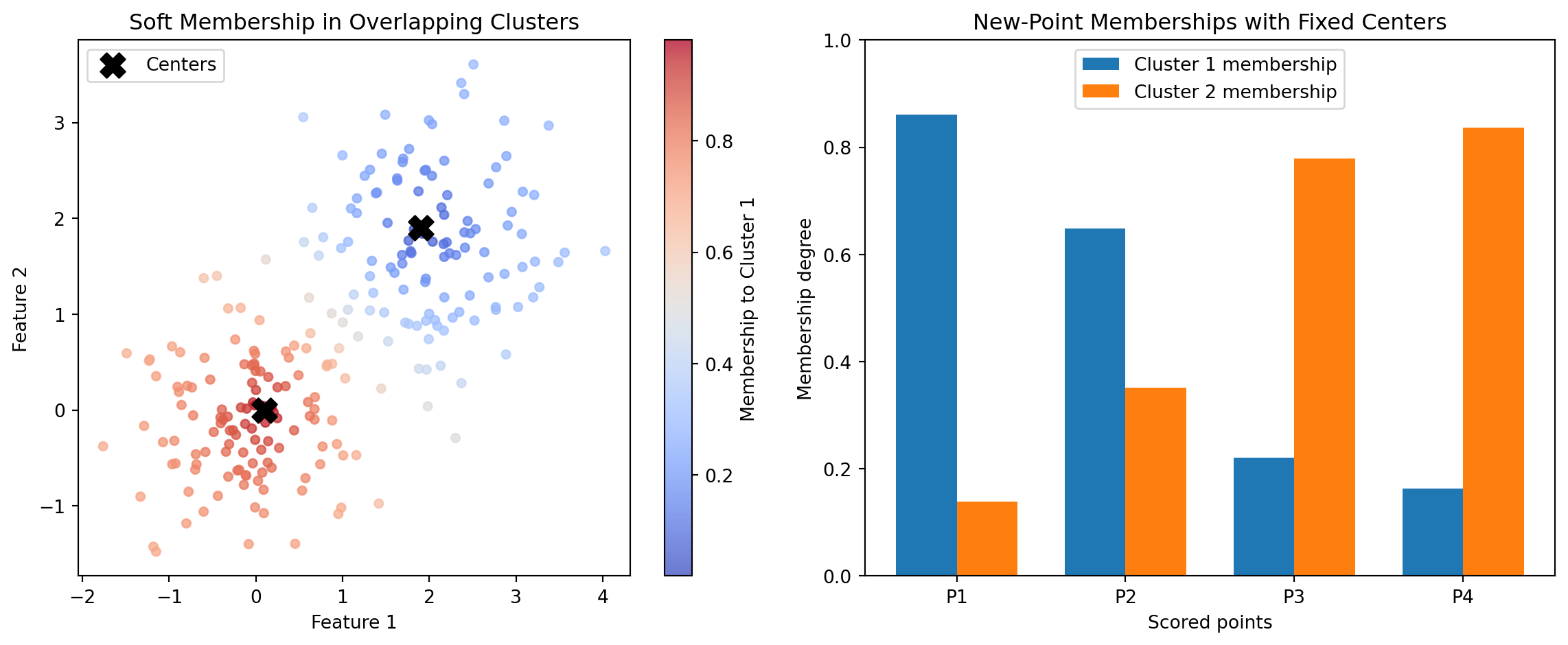
Traditional hard clustering (for example, k-means) answers: “Which single cluster does this point belong to?” Fuzzy c-means answers a richer question: “To what degree does this point belong to each cluster?” That distinction matters in many business and engineering domains where categories are inherently mixed. A customer can behave partly like a value buyer and partly like a premium buyer. A machine condition can be partly normal and partly degrading. A geographic zone can have mixed demand profiles. Soft membership captures this reality more faithfully.
From a mathematical perspective, fuzzy c-means optimizes cluster centers and a membership matrix simultaneously. The result includes:
- Cluster centers (
cntr) that represent typical patterns. - Membership matrix (
u) showing each point’s fractional affiliation with each cluster. - Distances (
d) from points to centers. - Objective history (
jm) and convergence state (p) used for diagnostics. - Fuzzy partition coefficient (
fpc) as a compact measure of partition sharpness.
From a practical perspective, these outputs support workflows that go beyond segmentation itself. Teams can rank records by cluster affinity, define soft thresholds for interventions, and monitor how memberships drift over time. This is why fuzzy clustering is useful not only for exploratory analysis but also for operational decision support.
Boardflare’s two calculators map directly to two phases of a clustering lifecycle:
- Model establishment with CMEANS: identify centers and baseline memberships from historical data.
- Model application with CMEANS_PREDICT: score new observations against fixed, previously trained centers.
This separation is important for controlled analytics. It lets teams train a reference clustering model, freeze its centers for governance, and then score incoming data consistently over time. That pattern is common in production analytics pipelines where model stability and auditability matter as much as raw fit.
When to Use It Use this category when the job is to uncover latent structure in unlabeled data and preserve nuance in category boundaries. In other words, use fuzzy clustering when real-world entities can plausibly belong to multiple groups at once.
One high-value scenario is customer and account segmentation in go-to-market analytics. Suppose a revenue operations team wants to segment accounts by product usage, support intensity, and spend trajectory. Hard segmentation can force an account into only one bucket, which often hides transition behavior. With CMEANS, analysts produce cluster centers and membership degrees that reveal blended profiles (for example, “70% growth-oriented, 30% cost-sensitive”). As new accounts arrive each week, CMEANS_PREDICT assigns memberships to those same strategic segments without retraining every time. This supports consistent routing, campaign personalization, and quarterly planning.
A second scenario is industrial condition monitoring. Sensors on pumps, compressors, or turbines rarely produce crisp, separable states. A machine can gradually transition from healthy to early-fault behavior. Fuzzy memberships are a natural fit because they quantify partial condition overlap. Engineers train baseline states with CMEANS, then score streaming batches with CMEANS_PREDICT to detect early drift. Rising membership in a “degradation” cluster can trigger preventive maintenance before hard alarm thresholds are reached.
A third scenario is supply and demand zoning in logistics or retail networks. Regional demand patterns are often mixtures: a zone may show both urban and suburban demand signatures depending on daypart and product mix. Hard clustering can produce brittle decisions when zones sit near boundaries. Fuzzy assignments from CMEANS let planners treat zones with mixed identity differently in inventory policies and staffing models. Then CMEANS_PREDICT maps new periods or new locations into the same framework for ongoing network calibration.
This category is also useful in risk analytics, healthcare stratification, and anomaly triage when stakeholders need explainable gradations instead of one-shot labels. The membership matrix becomes a decision surface: high-confidence cases can be auto-routed, while ambiguous cases receive human review.
Situations where fuzzy clustering is especially appropriate:
- Cluster overlap is expected and meaningful.
- Decision logic benefits from graded certainty.
- Teams need stable centers for future scoring.
- Analysts want both center-level summaries and record-level affinities.
Situations where it may be less appropriate:
- Data are strongly separable and hard labels are required for compliance logic.
- There is no tolerance for tuning hyperparameters such as fuzziness exponent
m. - Business process cannot consume probabilistic or fractional outputs.
In short, this category is best when the job is not just “group records,” but “characterize mixed membership in a reproducible way.”
How It Works The underlying method is fuzzy c-means optimization. Let x_j \in \mathbb{R}^d be data points, v_i be cluster centers for i=1,\dots,c, and u_{ij} be membership of point j in cluster i.
The core objective minimized by CMEANS is:
J_m(U, V) = \sum_{j=1}^{N} \sum_{i=1}^{c} u_{ij}^m \lVert x_j - v_i \rVert^2
subject to:
\sum_{i=1}^{c} u_{ij} = 1, \quad 0 \le u_{ij} \le 1
The exponent m > 1 controls fuzziness. As m \to 1, assignments become harder; larger m spreads membership more evenly across clusters.
The alternating updates are conceptually:
v_i = \frac{\sum_{j=1}^{N} u_{ij}^m x_j}{\sum_{j=1}^{N} u_{ij}^m}
and
u_{ij} = \left(\sum_{k=1}^{c} \left(\frac{\lVert x_j-v_i\rVert}{\lVert x_j-v_k\rVert}\right)^{\frac{2}{m-1}}\right)^{-1}
The algorithm iterates until either the membership matrix change falls below error or maxiter is reached. In Boardflare’s CMEANS, inputs are organized as features by samples, so shape conventions should be checked before use.
The key diagnostics include:
jm: objective function values across iterations, useful for confirming descent and convergence behavior.p: effective iteration count.fpc: fuzzy partition coefficient, often interpreted in [0,1] where higher values suggest crisper partitions.
For scoring new data, CMEANS_PREDICT keeps trained centers fixed and solves memberships for incoming points under the same fuzzy framework. Conceptually, this is the deployment step: no center re-estimation, only assignment against known prototypes. That distinction makes outputs comparable over time.
Why this matters operationally:
- Governance: fixed centers prevent silent drift from retraining on every batch.
- Consistency: weekly or daily scores remain anchored to the same segment definitions.
- Speed: prediction is lighter than full retraining when centers are already validated.
The upstream implementation is provided by scikit-fuzzy, with numerics based on NumPy/SciPy arrays. In Boardflare calculators, users provide structured arrays from spreadsheet-like inputs and receive dictionary outputs with both scalar and matrix fields.
Important assumptions and requirements:
- Distance is Euclidean in standard fuzzy c-means; feature scaling strongly affects results.
c(number of clusters) must be set by the analyst; it is not inferred automatically.mcontrols overlap; common starting value is around 2, then tuned by interpretability and stability.- Initialization can affect local minima, so sensitivity checks are good practice.
- Features should be normalized when units differ materially.
Compared with hard clustering, fuzzy c-means does not force a single segment identity. This is mathematically elegant and practically useful, but it also means downstream systems must know how to consume memberships. Typical strategies include maximum-membership assignment for simple routing, top-two memberships for mixed strategies, or threshold-based triage for uncertain records.
When interpreting results, teams should avoid over-reading tiny membership differences. For example, a record with memberships (0.51, 0.49) is intrinsically ambiguous and may warrant special handling. That ambiguity is a feature, not a bug: it surfaces uncertainty explicitly rather than hiding it.
Practical Example Consider a B2B SaaS team building account archetypes from three standardized signals: product usage intensity, support ticket load, and expansion propensity. The goal is to discover account segments and then score new accounts weekly for campaign and customer-success actions.
Step 1: Prepare a training matrix for CMEANS.
- Assemble historical account-level data.
- Standardize each feature so scale does not dominate distance.
- Arrange data in the calculator’s expected orientation (features x samples).
Step 2: Choose initial hyperparameters.
c = 3clusters for an initial business hypothesis (for example: growth, stable, at-risk).m = 2.0for moderate fuzziness.error = 0.005,maxiter = 100as practical convergence controls.
Step 3: Run CMEANS and inspect outputs.
Suppose the returned cntr suggests:
- Cluster A: high usage, moderate support, high expansion propensity.
- Cluster B: moderate usage, low support, stable expansion.
- Cluster C: low usage, high support, low expansion propensity.
The membership matrix u reveals mixed identities. An account might score 0.62 in Cluster A and 0.34 in Cluster B, indicating strong-but-not-exclusive growth behavior. Another might be 0.40 / 0.38 / 0.22, signaling ambiguity and a candidate for analyst review.
Step 4: Validate usefulness before operationalizing.
- Check whether clusters map to meaningful business actions.
- Review
fpcandjmtrends for quality and convergence. - Compare outcomes under nearby settings (for example,
c=4orm=1.8) to test stability.
Step 5: Freeze centers and transition to scoring mode with CMEANS_PREDICT.
- Store the validated
cntrmatrix as the reference segment definition. - For each new weekly batch, submit
test_dataandcntr_trained. - Receive updated memberships without changing the segment prototypes.
Step 6: Convert memberships into actions.
- If max membership \ge 0.75, route to segment-specific automation.
- If top-two memberships are close (for example, difference < 0.1), assign blended messaging.
- If all memberships are diffuse, route to manual strategy review.
Step 7: Monitor drift and retrain only when needed.
- Track distribution shifts in incoming feature data.
- Watch aggregate changes in membership patterns over time.
- Retrain with CMEANS on a defined cadence or when drift thresholds are breached.
This workflow is more effective than a traditional hard-assignment spreadsheet approach because it preserves uncertainty, supports transparent governance, and decouples model training from production scoring. The training/scoring split between CMEANS and CMEANS_PREDICT is exactly what enables repeatable operations.
How to Choose In this category, tool selection is straightforward and should align with lifecycle stage: train versus score.
- Choose CMEANS when cluster centers are unknown and must be learned from a representative dataset.
- Choose CMEANS_PREDICT when centers already exist and the task is to assign memberships for new observations consistently.
The decision process can be represented as:
graph TD
    A[Start: Need fuzzy cluster memberships] --> B{Do you already have trained centers?}
    B -- No --> C[Use CMEANS to learn centers and memberships]
    B -- Yes --> D[Use CMEANS_PREDICT to score new data]
    C --> E{Are segment definitions stable and approved?}
    E -- Yes --> D
    E -- No --> C
Comparison guidance:
| Function | Primary Job | Key Inputs | Main Outputs | Strengths | Trade-offs |
|---|---|---|---|---|---|
| CMEANS | Train fuzzy clusters | data, c, m, error, maxiter |
cntr, u, d, jm, p, fpc |
Learns structure from scratch; provides full diagnostics and centers | Requires hyperparameter tuning; retraining can change segment definitions |
| CMEANS_PREDICT | Score new points against fixed centers | test_data, cntr_trained, m, error, maxiter |
u, d, jm, p, fpc |
Consistent production scoring; no center drift during inference | Cannot discover new cluster structure; quality depends on trained centers |
A practical rule set for analysts:
- Begin with CMEANS during model development and periodic recalibration.
- Move to CMEANS_PREDICT for recurring operational scoring.
- Revisit CMEANS only when data drift, strategy shifts, or performance diagnostics justify retraining.
Parameter-selection tips across both tools:
- Cluster count (
c): start from business archetypes, then test interpretability and stability. - Fuzziness (
m): use around 2 as baseline; increase if memberships are too brittle, decrease if too diffuse. - Convergence controls (
error,maxiter): tighter error improves precision but can increase runtime. - Data orientation: ensure matrix shape is features x samples to match function expectations.
Common implementation mistakes and remedies:
- Mistake: interpreting low
fpcalone as model failure. Remedy: pair it with business interpretability and membership usability. - Mistake: retraining constantly and losing segment continuity. Remedy: separate training and scoring phases with center governance.
- Mistake: skipping feature scaling. Remedy: standardize before clustering to avoid unit-dominated distances.
If the business goal is exploratory discovery, prioritize CMEANS. If the goal is repeatable production assignment, prioritize CMEANS_PREDICT with validated centers. Most mature deployments use both in sequence: learn, govern, score, monitor, then retrain on policy.
AGGLOMERATIVE
Agglomerative clustering starts with each sample as its own cluster and repeatedly merges the closest pair according to a chosen linkage rule.
For example, Ward’s linkage (the default method) merges clusters A and B to minimize the increase in total within-cluster variance, evaluating distances as:
d(A, B) = \frac{|A| |B|}{|A| + |B|} ||\mu_A - \mu_B||^2
where \mu_A and \mu_B are the centroids of clusters A and B, respectively.
This wrapper accepts data with rows as samples and columns as features. It returns the final labels, a compact label count table, the merge tree children array, and optional merge distances when distance computation is enabled.
Excel Usage
=AGGLOMERATIVE(data, n_clusters, aggl_linkage, aggl_metric, compute_distances)data(list[list], required): 2D array of input data with rows as samples and columns as features.n_clusters(int, optional, default: 2): Number of clusters to keep after hierarchical merging.aggl_linkage(str, optional, default: “ward”): Linkage rule used when merging clusters.aggl_metric(str, optional, default: “euclidean”): Distance metric used when evaluating merges.compute_distances(bool, optional, default: false): Whether to store merge distances for the fitted tree.
Returns (dict): Excel data type containing the cluster count, labels, label counts, and hierarchical tree arrays.
Example 1: Form two clusters with Ward linkage on separated points
Inputs:
| data | n_clusters | aggl_linkage | aggl_metric | compute_distances | |
|---|---|---|---|---|---|
| 0 | 0 | 2 | ward | euclidean | false |
| 0 | 1 | ||||
| 1 | 0 | ||||
| 5 | 5 | ||||
| 5 | 6 | ||||
| 6 | 5 |
Excel formula:
=AGGLOMERATIVE({0,0;0,1;1,0;5,5;5,6;6,5}, 2, "ward", "euclidean", FALSE)Expected output:
{"type":"Double","basicValue":2,"properties":{"cluster_count":{"type":"Double","basicValue":2},"labels":{"type":"Array","elements":[[{"type":"Double","basicValue":1}],[{"type":"Double","basicValue":1}],[{"type":"Double","basicValue":1}],[{"type":"Double","basicValue":0}],[{"type":"Double","basicValue":0}],[{"type":"Double","basicValue":0}]]},"label_counts":{"type":"Array","elements":[[{"type":"String","basicValue":"label"},{"type":"String","basicValue":"count"}],[{"type":"Double","basicValue":0},{"type":"Double","basicValue":3}],[{"type":"Double","basicValue":1},{"type":"Double","basicValue":3}]]},"children":{"type":"Array","elements":[[{"type":"Double","basicValue":0},{"type":"Double","basicValue":1}],[{"type":"Double","basicValue":3},{"type":"Double","basicValue":4}],[{"type":"Double","basicValue":2},{"type":"Double","basicValue":6}],[{"type":"Double","basicValue":5},{"type":"Double","basicValue":7}],[{"type":"Double","basicValue":8},{"type":"Double","basicValue":9}]]},"n_leaves":{"type":"Double","basicValue":6},"n_connected_components":{"type":"Double","basicValue":1}}}
Example 2: Compute merge distances with average linkage and Manhattan distance
Inputs:
| data | n_clusters | aggl_linkage | aggl_metric | compute_distances | |
|---|---|---|---|---|---|
| 0 | 0 | 2 | average | manhattan | true |
| 0 | 1 | ||||
| 1 | 0 | ||||
| 6 | 6 | ||||
| 6 | 7 | ||||
| 7 | 6 |
Excel formula:
=AGGLOMERATIVE({0,0;0,1;1,0;6,6;6,7;7,6}, 2, "average", "manhattan", TRUE)Expected output:
{"type":"Double","basicValue":2,"properties":{"cluster_count":{"type":"Double","basicValue":2},"labels":{"type":"Array","elements":[[{"type":"Double","basicValue":1}],[{"type":"Double","basicValue":1}],[{"type":"Double","basicValue":1}],[{"type":"Double","basicValue":0}],[{"type":"Double","basicValue":0}],[{"type":"Double","basicValue":0}]]},"label_counts":{"type":"Array","elements":[[{"type":"String","basicValue":"label"},{"type":"String","basicValue":"count"}],[{"type":"Double","basicValue":0},{"type":"Double","basicValue":3}],[{"type":"Double","basicValue":1},{"type":"Double","basicValue":3}]]},"children":{"type":"Array","elements":[[{"type":"Double","basicValue":0},{"type":"Double","basicValue":1}],[{"type":"Double","basicValue":3},{"type":"Double","basicValue":4}],[{"type":"Double","basicValue":2},{"type":"Double","basicValue":6}],[{"type":"Double","basicValue":5},{"type":"Double","basicValue":7}],[{"type":"Double","basicValue":8},{"type":"Double","basicValue":9}]]},"n_leaves":{"type":"Double","basicValue":6},"n_connected_components":{"type":"Double","basicValue":1},"distances":{"type":"Array","elements":[[{"type":"Double","basicValue":1}],[{"type":"Double","basicValue":1}],[{"type":"Double","basicValue":1.5}],[{"type":"Double","basicValue":1.5}],[{"type":"Double","basicValue":12}]]}}}
Example 3: Merge one-dimensional samples with complete linkage and L1 distance
Inputs:
| data | n_clusters | aggl_linkage | aggl_metric | compute_distances |
|---|---|---|---|---|
| 0 | 2 | complete | l1 | false |
| 0.1 | ||||
| 0.2 | ||||
| 5 | ||||
| 5.1 | ||||
| 5.2 |
Excel formula:
=AGGLOMERATIVE({0;0.1;0.2;5;5.1;5.2}, 2, "complete", "l1", FALSE)Expected output:
{"type":"Double","basicValue":2,"properties":{"cluster_count":{"type":"Double","basicValue":2},"labels":{"type":"Array","elements":[[{"type":"Double","basicValue":1}],[{"type":"Double","basicValue":1}],[{"type":"Double","basicValue":1}],[{"type":"Double","basicValue":0}],[{"type":"Double","basicValue":0}],[{"type":"Double","basicValue":0}]]},"label_counts":{"type":"Array","elements":[[{"type":"String","basicValue":"label"},{"type":"String","basicValue":"count"}],[{"type":"Double","basicValue":0},{"type":"Double","basicValue":3}],[{"type":"Double","basicValue":1},{"type":"Double","basicValue":3}]]},"children":{"type":"Array","elements":[[{"type":"Double","basicValue":3},{"type":"Double","basicValue":4}],[{"type":"Double","basicValue":0},{"type":"Double","basicValue":1}],[{"type":"Double","basicValue":2},{"type":"Double","basicValue":7}],[{"type":"Double","basicValue":5},{"type":"Double","basicValue":6}],[{"type":"Double","basicValue":8},{"type":"Double","basicValue":9}]]},"n_leaves":{"type":"Double","basicValue":6},"n_connected_components":{"type":"Double","basicValue":1}}}
Example 4: Separate directional vectors with cosine single linkage
Inputs:
| data | n_clusters | aggl_linkage | aggl_metric | compute_distances | |
|---|---|---|---|---|---|
| 1 | 0 | 2 | single | cosine | true |
| 0.95 | 0.05 | ||||
| 0 | 1 | ||||
| 0.05 | 0.95 |
Excel formula:
=AGGLOMERATIVE({1,0;0.95,0.05;0,1;0.05,0.95}, 2, "single", "cosine", TRUE)Expected output:
{"type":"Double","basicValue":2,"properties":{"cluster_count":{"type":"Double","basicValue":2},"labels":{"type":"Array","elements":[[{"type":"Double","basicValue":1}],[{"type":"Double","basicValue":1}],[{"type":"Double","basicValue":0}],[{"type":"Double","basicValue":0}]]},"label_counts":{"type":"Array","elements":[[{"type":"String","basicValue":"label"},{"type":"String","basicValue":"count"}],[{"type":"Double","basicValue":0},{"type":"Double","basicValue":2}],[{"type":"Double","basicValue":1},{"type":"Double","basicValue":2}]]},"children":{"type":"Array","elements":[[{"type":"Double","basicValue":0},{"type":"Double","basicValue":1}],[{"type":"Double","basicValue":2},{"type":"Double","basicValue":3}],[{"type":"Double","basicValue":4},{"type":"Double","basicValue":5}]]},"n_leaves":{"type":"Double","basicValue":4},"n_connected_components":{"type":"Double","basicValue":1},"distances":{"type":"Array","elements":[[{"type":"Double","basicValue":0.00138217}],[{"type":"Double","basicValue":0.00138217}],[{"type":"Double","basicValue":0.895028}]]}}}
Python Code
Show Code
import numpy as np
from sklearn.cluster import AgglomerativeClustering as SklearnAgglomerativeClustering

def agglomerative(data, n_clusters=2, aggl_linkage='ward', aggl_metric='euclidean', compute_distances=False):
    """
    Build hierarchical clusters by recursively merging samples.

    See: https://scikit-learn.org/stable/modules/generated/sklearn.cluster.AgglomerativeClustering.html

    This example function is provided as-is without any representation of accuracy.

    Args:
        data (list[list]): 2D array of input data with rows as samples and columns as features.
        n_clusters (int, optional): Number of clusters to keep after hierarchical merging. Default is 2.
        aggl_linkage (str, optional): Linkage rule used when merging clusters. Valid options: Ward, Complete, Average, Single. Default is 'ward'.
        aggl_metric (str, optional): Distance metric used when evaluating merges. Valid options: Euclidean, Manhattan, L1, L2, Cosine. Default is 'euclidean'.
        compute_distances (bool, optional): Whether to store merge distances for the fitted tree. Default is False.

    Returns:
        dict: Excel data type containing the cluster count, labels, label counts, and hierarchical tree arrays.
    """
    def to2d(value):
        return [[value]] if not isinstance(value, list) else value

    def parse_matrix(value):
        value = to2d(value)
        if not isinstance(value, list) or not value or not all(isinstance(row, list) and row for row in value):
            return None, "Error: data must be a non-empty 2D list"
        if len({len(row) for row in value}) != 1:
            return None, "Error: data must be a rectangular 2D list"
        matrix = np.array(value, dtype=float)
        if matrix.ndim != 2 or matrix.size == 0:
            return None, "Error: data must be a non-empty 2D list"
        if not np.isfinite(matrix).all():
            return None, "Error: data must contain only finite numeric values"
        return matrix, None

    def as_column(values):
        return [[{"type": "Double", "basicValue": float(item)}] for item in values]

    def as_matrix(values):
        return [[{"type": "Double", "basicValue": float(item)} for item in row] for row in values]

    def label_count_table(labels):
        unique_labels, counts = np.unique(labels, return_counts=True)
        rows = [[{"type": "String", "basicValue": "label"}, {"type": "String", "basicValue": "count"}]]
        rows.extend(
            [[{"type": "Double", "basicValue": float(label)}, {"type": "Double", "basicValue": float(count)}]
             for label, count in zip(unique_labels.tolist(), counts.tolist())]
        )
        return rows

    try:
        data_np, error = parse_matrix(data)
        if error:
            return error

        cluster_total = int(n_clusters)
        if cluster_total < 1:
            return "Error: n_clusters must be at least 1"
        if cluster_total > data_np.shape[0]:
            return "Error: n_clusters cannot exceed the number of samples"

        linkage_value = str(aggl_linkage).strip()
        metric_value = str(aggl_metric).strip()
        if linkage_value not in {"ward", "complete", "average", "single"}:
            return "Error: linkage must be one of 'ward', 'complete', 'average', or 'single'"
        if metric_value not in {"euclidean", "manhattan", "l1", "l2", "cosine"}:
            return "Error: metric must be one of 'euclidean', 'manhattan', 'l1', 'l2', or 'cosine'"
        if linkage_value == "ward" and metric_value != "euclidean":
            return "Error: metric must be euclidean when linkage is ward"

        fitted = SklearnAgglomerativeClustering(
            n_clusters=cluster_total,
            linkage=linkage_value,
            metric=metric_value,
            compute_distances=bool(compute_distances)
        ).fit(data_np)

        labels = fitted.labels_
        properties = {
            "cluster_count": {"type": "Double", "basicValue": float(fitted.n_clusters_)},
            "labels": {"type": "Array", "elements": as_column(labels.tolist())},
            "label_counts": {"type": "Array", "elements": label_count_table(labels)},
            "children": {"type": "Array", "elements": as_matrix(fitted.children_.tolist())},
            "n_leaves": {"type": "Double", "basicValue": float(fitted.n_leaves_)},
            "n_connected_components": {"type": "Double", "basicValue": float(fitted.n_connected_components_)}
        }
        if hasattr(fitted, "distances_"):
            properties["distances"] = {"type": "Array", "elements": as_column(fitted.distances_.tolist())}

        return {
            "type": "Double",
            "basicValue": float(fitted.n_clusters_),
            "properties": properties
        }
    except Exception as e:
        return f"Error: {str(e)}"
Online Calculator
2D array of input data with rows as samples and columns as features.
Number of clusters to keep after hierarchical merging.
Linkage rule used when merging clusters.
Distance metric used when evaluating merges.
Whether to store merge distances for the fitted tree.
BIRCH_CLUSTER
BIRCH incrementally compresses samples into subclusters using a tree structure and then performs a final clustering step on those subcluster summaries.
It efficiently summarizes clusters using a Clustering Feature (CF), defined as a tuple:
CF = (N, \vec{LS}, SS)
where N is the number of data points in the cluster, \vec{LS} = \sum_{i=1}^{N} \vec{x}_i is the linear sum of the points, and SS = \sum_{i=1}^{N} ||\vec{x}_i||^2 is the sum of their squared norms.
This wrapper keeps label computation enabled and uses an integer final cluster count so the fitted result reliably includes labels, label counts, subcluster centers, and subcluster labels.
Excel Usage
=BIRCH_CLUSTER(data, threshold, branching_factor, n_clusters)data(list[list], required): 2D array of input data with rows as samples and columns as features.threshold(float, optional, default: 0.5): Maximum radius allowed when absorbing a sample into an existing subcluster.branching_factor(int, optional, default: 50): Maximum number of subclusters per node in the clustering tree.n_clusters(int, optional, default: 3): Number of final clusters formed from the learned subclusters.
Returns (dict): Excel data type containing final cluster counts, labels, label counts, and subcluster summaries.
Example 1: Cluster two compact groups with default BIRCH behavior
Inputs:
| data | threshold | branching_factor | n_clusters | |
|---|---|---|---|---|
| 0 | 0 | 0.5 | 50 | 2 |
| 0 | 1 | |||
| 1 | 0 | |||
| 5 | 5 | |||
| 5 | 6 | |||
| 6 | 5 |
Excel formula:
=BIRCH_CLUSTER({0,0;0,1;1,0;5,5;5,6;6,5}, 0.5, 50, 2)Expected output:
{"type":"Double","basicValue":2,"properties":{"cluster_count":{"type":"Double","basicValue":2},"subcluster_count":{"type":"Double","basicValue":4},"labels":{"type":"Array","elements":[[{"type":"Double","basicValue":1}],[{"type":"Double","basicValue":1}],[{"type":"Double","basicValue":1}],[{"type":"Double","basicValue":0}],[{"type":"Double","basicValue":0}],[{"type":"Double","basicValue":0}]]},"label_counts":{"type":"Array","elements":[[{"type":"String","basicValue":"label"},{"type":"String","basicValue":"count"}],[{"type":"Double","basicValue":0},{"type":"Double","basicValue":3}],[{"type":"Double","basicValue":1},{"type":"Double","basicValue":3}]]},"subcluster_centers":{"type":"Array","elements":[[{"type":"Double","basicValue":0},{"type":"Double","basicValue":0.5}],[{"type":"Double","basicValue":1},{"type":"Double","basicValue":0}],[{"type":"Double","basicValue":5},{"type":"Double","basicValue":5.5}],[{"type":"Double","basicValue":6},{"type":"Double","basicValue":5}]]},"subcluster_labels":{"type":"Array","elements":[[{"type":"Double","basicValue":1}],[{"type":"Double","basicValue":1}],[{"type":"Double","basicValue":0}],[{"type":"Double","basicValue":0}]]}}}
Example 2: Summarize three compact groups into final clusters
Inputs:
| data | threshold | branching_factor | n_clusters | |
|---|---|---|---|---|
| 1 | 1 | 0.4 | 20 | 3 |
| 1.2 | 0.8 | |||
| 0.8 | 1.1 | |||
| 8 | 8 | |||
| 8.2 | 7.9 | |||
| 7.8 | 8.1 | |||
| 15 | 1 | |||
| 15.2 | 0.8 | |||
| 14.8 | 1.1 |
Excel formula:
=BIRCH_CLUSTER({1,1;1.2,0.8;0.8,1.1;8,8;8.2,7.9;7.8,8.1;15,1;15.2,0.8;14.8,1.1}, 0.4, 20, 3)Expected output:
{"type":"Double","basicValue":3,"properties":{"cluster_count":{"type":"Double","basicValue":3},"subcluster_count":{"type":"Double","basicValue":3},"labels":{"type":"Array","elements":[[{"type":"Double","basicValue":2}],[{"type":"Double","basicValue":2}],[{"type":"Double","basicValue":2}],[{"type":"Double","basicValue":1}],[{"type":"Double","basicValue":1}],[{"type":"Double","basicValue":1}],[{"type":"Double","basicValue":0}],[{"type":"Double","basicValue":0}],[{"type":"Double","basicValue":0}]]},"label_counts":{"type":"Array","elements":[[{"type":"String","basicValue":"label"},{"type":"String","basicValue":"count"}],[{"type":"Double","basicValue":0},{"type":"Double","basicValue":3}],[{"type":"Double","basicValue":1},{"type":"Double","basicValue":3}],[{"type":"Double","basicValue":2},{"type":"Double","basicValue":3}]]},"subcluster_centers":{"type":"Array","elements":[[{"type":"Double","basicValue":1},{"type":"Double","basicValue":0.966667}],[{"type":"Double","basicValue":8},{"type":"Double","basicValue":8}],[{"type":"Double","basicValue":15},{"type":"Double","basicValue":0.966667}]]},"subcluster_labels":{"type":"Array","elements":[[{"type":"Double","basicValue":2}],[{"type":"Double","basicValue":1}],[{"type":"Double","basicValue":0}]]}}}
Example 3: Cluster a single Excel cell into one BIRCH cluster
Inputs:
| data | threshold | branching_factor | n_clusters |
|---|---|---|---|
| 5 | 0.5 | 10 | 1 |
Excel formula:
=BIRCH_CLUSTER(5, 0.5, 10, 1)Expected output:
{"type":"Double","basicValue":1,"properties":{"cluster_count":{"type":"Double","basicValue":1},"subcluster_count":{"type":"Double","basicValue":1},"labels":{"type":"Array","elements":[[{"type":"Double","basicValue":0}]]},"label_counts":{"type":"Array","elements":[[{"type":"String","basicValue":"label"},{"type":"String","basicValue":"count"}],[{"type":"Double","basicValue":0},{"type":"Double","basicValue":1}]]},"subcluster_centers":{"type":"Array","elements":[[{"type":"Double","basicValue":5}]]},"subcluster_labels":{"type":"Array","elements":[[{"type":"Double","basicValue":0}]]}}}
Example 4: Build BIRCH clusters for one-dimensional samples
Inputs:
| data | threshold | branching_factor | n_clusters |
|---|---|---|---|
| 0 | 0.2 | 10 | 2 |
| 0.1 | |||
| 0.2 | |||
| 4.8 | |||
| 5 | |||
| 5.2 |
Excel formula:
=BIRCH_CLUSTER({0;0.1;0.2;4.8;5;5.2}, 0.2, 10, 2)Expected output:
{"type":"Double","basicValue":2,"properties":{"cluster_count":{"type":"Double","basicValue":2},"subcluster_count":{"type":"Double","basicValue":2},"labels":{"type":"Array","elements":[[{"type":"Double","basicValue":1}],[{"type":"Double","basicValue":1}],[{"type":"Double","basicValue":1}],[{"type":"Double","basicValue":0}],[{"type":"Double","basicValue":0}],[{"type":"Double","basicValue":0}]]},"label_counts":{"type":"Array","elements":[[{"type":"String","basicValue":"label"},{"type":"String","basicValue":"count"}],[{"type":"Double","basicValue":0},{"type":"Double","basicValue":3}],[{"type":"Double","basicValue":1},{"type":"Double","basicValue":3}]]},"subcluster_centers":{"type":"Array","elements":[[{"type":"Double","basicValue":0.1}],[{"type":"Double","basicValue":5}]]},"subcluster_labels":{"type":"Array","elements":[[{"type":"Double","basicValue":1}],[{"type":"Double","basicValue":0}]]}}}
Python Code
Show Code
import numpy as np
from sklearn.cluster import Birch as SklearnBirch

def birch_cluster(data, threshold=0.5, branching_factor=50, n_clusters=3):
    """
    Cluster samples with the BIRCH incremental clustering algorithm.

    See: https://scikit-learn.org/stable/modules/generated/sklearn.cluster.Birch.html

    This example function is provided as-is without any representation of accuracy.

    Args:
        data (list[list]): 2D array of input data with rows as samples and columns as features.
        threshold (float, optional): Maximum radius allowed when absorbing a sample into an existing subcluster. Default is 0.5.
        branching_factor (int, optional): Maximum number of subclusters per node in the clustering tree. Default is 50.
        n_clusters (int, optional): Number of final clusters formed from the learned subclusters. Default is 3.

    Returns:
        dict: Excel data type containing final cluster counts, labels, label counts, and subcluster summaries.
    """
    def to2d(value):
        return [[value]] if not isinstance(value, list) else value

    def parse_matrix(value):
        value = to2d(value)
        if not isinstance(value, list) or not value or not all(isinstance(row, list) and row for row in value):
            return None, "Error: data must be a non-empty 2D list"
        if len({len(row) for row in value}) != 1:
            return None, "Error: data must be a rectangular 2D list"
        matrix = np.array(value, dtype=float)
        if matrix.ndim != 2 or matrix.size == 0:
            return None, "Error: data must be a non-empty 2D list"
        if not np.isfinite(matrix).all():
            return None, "Error: data must contain only finite numeric values"
        return matrix, None

    def as_column(values):
        return [[{"type": "Double", "basicValue": float(item)}] for item in values]

    def as_matrix(values):
        return [[{"type": "Double", "basicValue": float(item)} for item in row] for row in values]

    def label_count_table(labels):
        unique_labels, counts = np.unique(labels, return_counts=True)
        rows = [[{"type": "String", "basicValue": "label"}, {"type": "String", "basicValue": "count"}]]
        rows.extend(
            [[{"type": "Double", "basicValue": float(label)}, {"type": "Double", "basicValue": float(count)}]
             for label, count in zip(unique_labels.tolist(), counts.tolist())]
        )
        return rows

    try:
        data_np, error = parse_matrix(data)
        if error:
            return error

        if float(threshold) <= 0:
            return "Error: threshold must be greater than 0"
        if int(branching_factor) < 2:
            return "Error: branching_factor must be at least 2"

        cluster_total = int(n_clusters)
        if cluster_total < 1:
            return "Error: n_clusters must be at least 1"
        if cluster_total > data_np.shape[0]:
            return "Error: n_clusters cannot exceed the number of samples"

        if data_np.shape[0] == 1 and cluster_total == 1:
            labels = np.array([0])
            return {
                "type": "Double",
                "basicValue": 1.0,
                "properties": {
                    "cluster_count": {"type": "Double", "basicValue": 1.0},
                    "subcluster_count": {"type": "Double", "basicValue": 1.0},
                    "labels": {"type": "Array", "elements": as_column(labels.tolist())},
                    "label_counts": {"type": "Array", "elements": label_count_table(labels)},
                    "subcluster_centers": {"type": "Array", "elements": as_matrix(data_np.tolist())},
                    "subcluster_labels": {"type": "Array", "elements": as_column(labels.tolist())}
                }
            }

        fitted = SklearnBirch(
            threshold=float(threshold),
            branching_factor=int(branching_factor),
            n_clusters=cluster_total,
            compute_labels=True
        ).fit(data_np)

        labels = fitted.labels_
        cluster_count = int(np.unique(labels).size)
        subcluster_total = int(len(fitted.subcluster_centers_))

        return {
            "type": "Double",
            "basicValue": float(cluster_count),
            "properties": {
                "cluster_count": {"type": "Double", "basicValue": float(cluster_count)},
                "subcluster_count": {"type": "Double", "basicValue": float(subcluster_total)},
                "labels": {"type": "Array", "elements": as_column(labels.tolist())},
                "label_counts": {"type": "Array", "elements": label_count_table(labels)},
                "subcluster_centers": {"type": "Array", "elements": as_matrix(fitted.subcluster_centers_.tolist())},
                "subcluster_labels": {"type": "Array", "elements": as_column(fitted.subcluster_labels_.tolist())}
            }
        }
    except Exception as e:
        return f"Error: {str(e)}"
Online Calculator
2D array of input data with rows as samples and columns as features.
Maximum radius allowed when absorbing a sample into an existing subcluster.
Maximum number of subclusters per node in the clustering tree.
Number of final clusters formed from the learned subclusters.
CMEANS
Fuzzy c-means clustering allows each data point to belong to multiple clusters with varying degrees of membership. This is a soft clustering approach compared to k-means where each data point belongs to exactly one cluster.
The algorithm minimizes the following objective function:
J_m = \sum_{i=1}^{N} \sum_{j=1}^{C} u_{ij}^m ||x_i - c_j||^2
where N is the number of samples, C is the number of clusters, u_{ij} is the degree of membership of x_i in the cluster j, c_j is the cluster center, and m is the fuzziness parameter.
The algorithm handles high-dimensional datasets and overlapping clusters well, returning properties like the cluster centers, partition matrix, and objective function history.
Excel Usage
=CMEANS(data, c, m, error, maxiter)data(list[list], required): 2D array of data to be clustered, where rows are features and columns are samples (S x N). Note the transpose requirement compared to typical scikit-learn S x N layout.c(int, required): Desired number of clusters or classes.m(float, required): Array exponentiation applied to the membership function (fuzziness parameter, typically 2.0).error(float, required): Stopping criterion; stop early if the change in partition matrix is less than this error (e.g., 0.005).maxiter(int, required): Maximum number of iterations allowed.
Returns (dict): Dictionary of clustering results, including cluster centers and the fuzzy partition matrix.
Example 1: Fuzzy c-means clustering of 2D data
Inputs:
| data | c | m | error | maxiter | |
|---|---|---|---|---|---|
| 1 | 2 | 1 | 2 | 0.005 | 2 |
| 1 | 2 |
Excel formula:
=CMEANS({1,2;1,2}, 1, 2, 0.005, 2)Expected output:
{"type":"Double","basicValue":1,"properties":{"fpc":{"type":"Double","basicValue":1},"cntr":{"type":"Array","elements":[[{"type":"Double","basicValue":1.5},{"type":"Double","basicValue":1.5}]]},"u":{"type":"Array","elements":[[{"type":"Double","basicValue":1},{"type":"Double","basicValue":1}]]},"d":{"type":"Array","elements":[[{"type":"Double","basicValue":0.707107},{"type":"Double","basicValue":0.707107}]]},"jm":{"type":"Array","elements":[[{"type":"Double","basicValue":1}]]},"p":{"type":"Double","basicValue":1}}}
Python Code
Show Code
import numpy as np
from skfuzzy import cmeans as fuzz_cmeans

def cmeans(data, c, m, error, maxiter):
    """
    Perform fuzzy c-means clustering on data.

    See: https://pythonhosted.org/scikit-fuzzy/api/skfuzzy.html#skfuzzy.cmeans

    This example function is provided as-is without any representation of accuracy.

    Args:
        data (list[list]): 2D array of data to be clustered, where rows are features and columns are samples (S x N). Note the transpose requirement compared to typical scikit-learn S x N layout.
        c (int): Desired number of clusters or classes.
        m (float): Array exponentiation applied to the membership function (fuzziness parameter, typically 2.0).
        error (float): Stopping criterion; stop early if the change in partition matrix is less than this error (e.g., 0.005).
        maxiter (int): Maximum number of iterations allowed.

    Returns:
        dict: Dictionary of clustering results, including cluster centers and the fuzzy partition matrix.
    """
    try:
        data_np = np.array(data, dtype=float)
        if data_np.ndim != 2:
            return "Error: data must be a 2D array"

        cntr, u, u0, d, jm, p, fpc = fuzz_cmeans(
            data=data_np,
            c=c,
            m=m,
            error=error,
            maxiter=maxiter
        )

        return {
            "type": "Double",
            "basicValue": float(fpc),
            "properties": {
                "fpc": {"type": "Double", "basicValue": float(fpc)},
                "cntr": {
                    "type": "Array",
                    "elements": [[{"type": "Double", "basicValue": float(val)} for val in row] for row in cntr]
                },
                "u": {
                    "type": "Array",
                    "elements": [[{"type": "Double", "basicValue": float(val)} for val in row] for row in u]
                },
                "d": {
                    "type": "Array",
                    "elements": [[{"type": "Double", "basicValue": float(val)} for val in row] for row in d]
                },
                "jm": {
                    "type": "Array",
                    "elements": [[{"type": "Double", "basicValue": float(val)}] for val in jm]
                },
                "p": {"type": "Double", "basicValue": float(p)}
            }
        }
    except Exception as e:
        return f"Error: {str(e)}"
Online Calculator
2D array of data to be clustered, where rows are features and columns are samples (S x N). Note the transpose requirement compared to typical scikit-learn S x N layout.
Desired number of clusters or classes.
Array exponentiation applied to the membership function (fuzziness parameter, typically 2.0).
Stopping criterion; stop early if the change in partition matrix is less than this error (e.g., 0.005).
Maximum number of iterations allowed.
CMEANS_PREDICT
Prediction of new data in a given trained fuzzy c-means framework. This algorithm repeats the clustering with fixed cluster centers efficiently finding the fuzzy membership of all data points.
It computes the membership u_{ij} of a new data point x_i to an existing cluster center c_j using the formula:
u_{ij} = \frac{1}{\sum_{k=1}^{C} \left(\frac{||x_i - c_j||}{||x_i - c_k||}\right)^{\frac{2}{m-1}}}
where C is the total number of clusters, and m is the fuzziness parameter.
Excel Usage
=CMEANS_PREDICT(test_data, cntr_trained, m, error, maxiter)test_data(list[list], required): 2D array of new data to predict (features x samples S x N).cntr_trained(list[list], required): Location of trained centers from prior training c-means.m(float, required): Array exponentiation applied to the membership function.error(float, required): Stopping criterion.maxiter(int, required): Maximum number of iterations allowed.
Returns (dict): Dictionary of prediction results, including the fuzzy partition matrix.
Example 1: Fuzzy c-means prediction on new data
Inputs:
| test_data | cntr_trained | m | error | maxiter | ||
|---|---|---|---|---|---|---|
| 1.5 | 8.5 | 1.5 | 1.5 | 2 | 0.005 | 2 |
| 1.5 | 8.5 | 8.5 | 8.5 |
Excel formula:
=CMEANS_PREDICT({1.5,8.5;1.5,8.5}, {1.5,1.5;8.5,8.5}, 2, 0.005, 2)Expected output:
{"type":"Double","basicValue":1,"properties":{"fpc":{"type":"Double","basicValue":1},"u":{"type":"Array","elements":[[{"type":"Double","basicValue":1},{"type":"Double","basicValue":4.93038e-32}],[{"type":"Double","basicValue":4.93038e-32},{"type":"Double","basicValue":1}]]},"d":{"type":"Array","elements":[[{"type":"Double","basicValue":2.22045e-16},{"type":"Double","basicValue":9.89949}],[{"type":"Double","basicValue":9.89949},{"type":"Double","basicValue":2.22045e-16}]]},"jm":{"type":"Array","elements":[[{"type":"Double","basicValue":56.0623}],[{"type":"Double","basicValue":9.76215e-30}]]},"p":{"type":"Double","basicValue":2}}}
Python Code
Show Code
import numpy as np
from skfuzzy import cmeans_predict as fuzz_cmeans_predict

def cmeans_predict(test_data, cntr_trained, m, error, maxiter):
    """
    Predict cluster membership for new data given a trained fuzzy c-means model.

    See: https://pythonhosted.org/scikit-fuzzy/api/skfuzzy.html#skfuzzy.cmeans_predict

    This example function is provided as-is without any representation of accuracy.

    Args:
        test_data (list[list]): 2D array of new data to predict (features x samples S x N).
        cntr_trained (list[list]): Location of trained centers from prior training c-means.
        m (float): Array exponentiation applied to the membership function.
        error (float): Stopping criterion.
        maxiter (int): Maximum number of iterations allowed.

    Returns:
        dict: Dictionary of prediction results, including the fuzzy partition matrix.
    """
    try:
        test_data_np = np.array(test_data, dtype=float)
        if test_data_np.ndim != 2:
            return "Error: test_data must be a 2D array"

        cntr_trained_np = np.array(cntr_trained, dtype=float)

        u, u0, d, jm, p, fpc = fuzz_cmeans_predict(
            test_data=test_data_np,
            cntr_trained=cntr_trained_np,
            m=m,
            error=error,
            maxiter=maxiter
        )

        return {
            "type": "Double",
            "basicValue": float(fpc),
            "properties": {
                "fpc": {"type": "Double", "basicValue": float(fpc)},
                "u": {
                    "type": "Array",
                    "elements": [[{"type": "Double", "basicValue": float(val)} for val in row] for row in u]
                },
                "d": {
                    "type": "Array",
                    "elements": [[{"type": "Double", "basicValue": float(val)} for val in row] for row in d]
                },
                "jm": {
                    "type": "Array",
                    "elements": [[{"type": "Double", "basicValue": float(val)}] for val in jm]
                },
                "p": {"type": "Double", "basicValue": float(p)}
            }
        }
    except Exception as e:
        return f"Error: {str(e)}"
Online Calculator
2D array of new data to predict (features x samples S x N).
Location of trained centers from prior training c-means.
Array exponentiation applied to the membership function.
Stopping criterion.
Maximum number of iterations allowed.
DBSCAN
DBSCAN groups samples into dense regions without requiring a fixed cluster count in advance. Samples that do not belong to any dense region are labeled as noise.
The algorithm is based on the concept of an \epsilon-neighborhood for a given point x:
N_{\epsilon}(x) = \{ y \in D \mid \text{dist}(x, y) \le \epsilon \}
A point x is considered a core point if the number of points in its neighborhood is at least min_samples (i.e., |N_{\epsilon}(x)| \ge \text{min\_samples}).
This wrapper accepts data with rows as samples and columns as features. It returns fitted labels, a compact label count table, the number of discovered clusters excluding noise, and the number of noise points.
Excel Usage
=DBSCAN(data, eps, min_samples, dbscan_metric)data(list[list], required): 2D array of input data with rows as samples and columns as features.eps(float, optional, default: 0.5): Maximum neighborhood radius for connecting nearby samples.min_samples(int, optional, default: 5): Minimum neighborhood size needed for a core sample.dbscan_metric(str, optional, default: “euclidean”): Distance metric used to measure neighborhood reachability.
Returns (dict): Excel data type containing cluster counts, labels, label counts, and core sample indices.
Example 1: Detect two dense groups and one noise point
Inputs:
| data | eps | min_samples | dbscan_metric | |
|---|---|---|---|---|
| 0 | 0 | 0.25 | 2 | euclidean |
| 0 | 0.1 | |||
| 5 | 5 | |||
| 5.1 | 5 | |||
| 10 | 10 |
Excel formula:
=DBSCAN({0,0;0,0.1;5,5;5.1,5;10,10}, 0.25, 2, "euclidean")Expected output:
{"type":"Double","basicValue":2,"properties":{"cluster_count":{"type":"Double","basicValue":2},"noise_count":{"type":"Double","basicValue":1},"core_sample_count":{"type":"Double","basicValue":4},"labels":{"type":"Array","elements":[[{"type":"Double","basicValue":0}],[{"type":"Double","basicValue":0}],[{"type":"Double","basicValue":1}],[{"type":"Double","basicValue":1}],[{"type":"Double","basicValue":-1}]]},"label_counts":{"type":"Array","elements":[[{"type":"String","basicValue":"label"},{"type":"String","basicValue":"count"}],[{"type":"Double","basicValue":-1},{"type":"Double","basicValue":1}],[{"type":"Double","basicValue":0},{"type":"Double","basicValue":2}],[{"type":"Double","basicValue":1},{"type":"Double","basicValue":2}]]},"core_sample_indices":{"type":"Array","elements":[[{"type":"Double","basicValue":0}],[{"type":"Double","basicValue":1}],[{"type":"Double","basicValue":2}],[{"type":"Double","basicValue":3}]]}}}
Example 2: Treat a single Excel cell as one dense sample
Inputs:
| data | eps | min_samples | dbscan_metric |
|---|---|---|---|
| 5 | 0.5 | 1 | euclidean |
Excel formula:
=DBSCAN(5, 0.5, 1, "euclidean")Expected output:
{"type":"Double","basicValue":1,"properties":{"cluster_count":{"type":"Double","basicValue":1},"noise_count":{"type":"Double","basicValue":0},"core_sample_count":{"type":"Double","basicValue":1},"labels":{"type":"Array","elements":[[{"type":"Double","basicValue":0}]]},"label_counts":{"type":"Array","elements":[[{"type":"String","basicValue":"label"},{"type":"String","basicValue":"count"}],[{"type":"Double","basicValue":0},{"type":"Double","basicValue":1}]]},"core_sample_indices":{"type":"Array","elements":[[{"type":"Double","basicValue":0}]]}}}
Example 3: Use Manhattan distance for two rectangular groups
Inputs:
| data | eps | min_samples | dbscan_metric | |
|---|---|---|---|---|
| 0 | 0 | 1.5 | 2 | manhattan |
| 0 | 1 | |||
| 0 | 2 | |||
| 6 | 6 | |||
| 6 | 7 | |||
| 12 | 12 |
Excel formula:
=DBSCAN({0,0;0,1;0,2;6,6;6,7;12,12}, 1.5, 2, "manhattan")Expected output:
{"type":"Double","basicValue":2,"properties":{"cluster_count":{"type":"Double","basicValue":2},"noise_count":{"type":"Double","basicValue":1},"core_sample_count":{"type":"Double","basicValue":5},"labels":{"type":"Array","elements":[[{"type":"Double","basicValue":0}],[{"type":"Double","basicValue":0}],[{"type":"Double","basicValue":0}],[{"type":"Double","basicValue":1}],[{"type":"Double","basicValue":1}],[{"type":"Double","basicValue":-1}]]},"label_counts":{"type":"Array","elements":[[{"type":"String","basicValue":"label"},{"type":"String","basicValue":"count"}],[{"type":"Double","basicValue":-1},{"type":"Double","basicValue":1}],[{"type":"Double","basicValue":0},{"type":"Double","basicValue":3}],[{"type":"Double","basicValue":1},{"type":"Double","basicValue":2}]]},"core_sample_indices":{"type":"Array","elements":[[{"type":"Double","basicValue":0}],[{"type":"Double","basicValue":1}],[{"type":"Double","basicValue":2}],[{"type":"Double","basicValue":3}],[{"type":"Double","basicValue":4}]]}}}
Example 4: Cluster one-dimensional samples with the L1 metric
Inputs:
| data | eps | min_samples | dbscan_metric |
|---|---|---|---|
| 0 | 0.25 | 2 | l1 |
| 0.1 | |||
| 0.2 | |||
| 4.8 | |||
| 5 | |||
| 8 |
Excel formula:
=DBSCAN({0;0.1;0.2;4.8;5;8}, 0.25, 2, "l1")Expected output:
{"type":"Double","basicValue":2,"properties":{"cluster_count":{"type":"Double","basicValue":2},"noise_count":{"type":"Double","basicValue":1},"core_sample_count":{"type":"Double","basicValue":5},"labels":{"type":"Array","elements":[[{"type":"Double","basicValue":0}],[{"type":"Double","basicValue":0}],[{"type":"Double","basicValue":0}],[{"type":"Double","basicValue":1}],[{"type":"Double","basicValue":1}],[{"type":"Double","basicValue":-1}]]},"label_counts":{"type":"Array","elements":[[{"type":"String","basicValue":"label"},{"type":"String","basicValue":"count"}],[{"type":"Double","basicValue":-1},{"type":"Double","basicValue":1}],[{"type":"Double","basicValue":0},{"type":"Double","basicValue":3}],[{"type":"Double","basicValue":1},{"type":"Double","basicValue":2}]]},"core_sample_indices":{"type":"Array","elements":[[{"type":"Double","basicValue":0}],[{"type":"Double","basicValue":1}],[{"type":"Double","basicValue":2}],[{"type":"Double","basicValue":3}],[{"type":"Double","basicValue":4}]]}}}
Python Code
Show Code
import numpy as np
from sklearn.cluster import DBSCAN as SklearnDBSCAN

def dbscan(data, eps=0.5, min_samples=5, dbscan_metric='euclidean'):
    """
    Cluster samples by density and mark outliers as noise.

    See: https://scikit-learn.org/stable/modules/generated/sklearn.cluster.DBSCAN.html

    This example function is provided as-is without any representation of accuracy.

    Args:
        data (list[list]): 2D array of input data with rows as samples and columns as features.
        eps (float, optional): Maximum neighborhood radius for connecting nearby samples. Default is 0.5.
        min_samples (int, optional): Minimum neighborhood size needed for a core sample. Default is 5.
        dbscan_metric (str, optional): Distance metric used to measure neighborhood reachability. Valid options: Euclidean, Manhattan, L1, L2, Cosine. Default is 'euclidean'.

    Returns:
        dict: Excel data type containing cluster counts, labels, label counts, and core sample indices.
    """
    def to2d(value):
        return [[value]] if not isinstance(value, list) else value

    def parse_matrix(value):
        value = to2d(value)
        if not isinstance(value, list) or not value or not all(isinstance(row, list) and row for row in value):
            return None, "Error: data must be a non-empty 2D list"
        if len({len(row) for row in value}) != 1:
            return None, "Error: data must be a rectangular 2D list"
        matrix = np.array(value, dtype=float)
        if matrix.ndim != 2 or matrix.size == 0:
            return None, "Error: data must be a non-empty 2D list"
        if not np.isfinite(matrix).all():
            return None, "Error: data must contain only finite numeric values"
        return matrix, None

    def as_column(values):
        return [[{"type": "Double", "basicValue": float(item)}] for item in values]

    def label_count_table(labels):
        unique_labels, counts = np.unique(labels, return_counts=True)
        rows = [[{"type": "String", "basicValue": "label"}, {"type": "String", "basicValue": "count"}]]
        rows.extend(
            [[{"type": "Double", "basicValue": float(label)}, {"type": "Double", "basicValue": float(count)}]
             for label, count in zip(unique_labels.tolist(), counts.tolist())]
        )
        return rows

    try:
        data_np, error = parse_matrix(data)
        if error:
            return error

        if float(eps) <= 0:
            return "Error: eps must be greater than 0"
        if int(min_samples) < 1:
            return "Error: min_samples must be at least 1"

        metric_value = str(dbscan_metric).strip()
        if metric_value not in {"euclidean", "manhattan", "l1", "l2", "cosine"}:
            return "Error: metric must be one of 'euclidean', 'manhattan', 'l1', 'l2', or 'cosine'"

        fitted = SklearnDBSCAN(
            eps=float(eps),
            min_samples=int(min_samples),
            metric=metric_value
        ).fit(data_np)

        labels = fitted.labels_
        noise_count = int(np.sum(labels == -1))
        cluster_count = int(len([label for label in np.unique(labels).tolist() if label != -1]))
        properties = {
            "cluster_count": {"type": "Double", "basicValue": float(cluster_count)},
            "noise_count": {"type": "Double", "basicValue": float(noise_count)},
            "core_sample_count": {"type": "Double", "basicValue": float(len(fitted.core_sample_indices_))},
            "labels": {"type": "Array", "elements": as_column(labels.tolist())},
            "label_counts": {"type": "Array", "elements": label_count_table(labels)}
        }

        if len(fitted.core_sample_indices_) > 0:
            properties["core_sample_indices"] = {"type": "Array", "elements": as_column(fitted.core_sample_indices_.tolist())}

        return {
            "type": "Double",
            "basicValue": float(cluster_count),
            "properties": properties
        }
    except Exception as e:
        return f"Error: {str(e)}"
Online Calculator
2D array of input data with rows as samples and columns as features.
Maximum neighborhood radius for connecting nearby samples.
Minimum neighborhood size needed for a core sample.
Distance metric used to measure neighborhood reachability.
KMEANS
K-means clustering partitions a set of samples into a fixed number of clusters by iteratively assigning each sample to the nearest centroid and then recomputing the centroid positions.
The algorithm minimizes the within-cluster sum of squares (inertia), defined as:
J = \sum_{j=1}^{k} \sum_{x_i \in S_j} ||x_i - \mu_j||^2
where k is the number of clusters, S_j is the j-th cluster, and \mu_j is the centroid of S_j.
This wrapper accepts data with rows as samples and columns as features. It returns the fitted labels, a compact label count table, the learned cluster centers, and the final inertia, which is the sum of squared distances from each sample to its assigned centroid.
Excel Usage
=KMEANS(data, n_clusters, kmeans_init, max_iter, tol, random_state)data(list[list], required): 2D array of input data with rows as samples and columns as features.n_clusters(int, optional, default: 8): Number of clusters to fit.kmeans_init(str, optional, default: “k-means++”): Initialization method for the starting centroids.max_iter(int, optional, default: 300): Maximum number of k-means iterations.tol(float, optional, default: 0.0001): Relative tolerance for declaring convergence.random_state(int, optional, default: null): Integer seed for reproducible centroid initialization. Leave blank for non-deterministic runs.
Returns (dict): Excel data type containing inertia, labels, label counts, and cluster centers.
Example 1: Separate two compact point clouds with k-means++
Inputs:
| data | n_clusters | kmeans_init | max_iter | tol | random_state | |
|---|---|---|---|---|---|---|
| 0 | 0 | 2 | k-means++ | 300 | 0.0001 | 0 |
| 0 | 1 | |||||
| 1 | 0 | |||||
| 5 | 5 | |||||
| 5 | 6 | |||||
| 6 | 5 |
Excel formula:
=KMEANS({0,0;0,1;1,0;5,5;5,6;6,5}, 2, "k-means++", 300, 0.0001, 0)Expected output:
{"type":"Double","basicValue":2.66667,"properties":{"inertia":{"type":"Double","basicValue":2.66667},"cluster_count":{"type":"Double","basicValue":2},"labels":{"type":"Array","elements":[[{"type":"Double","basicValue":1}],[{"type":"Double","basicValue":1}],[{"type":"Double","basicValue":1}],[{"type":"Double","basicValue":0}],[{"type":"Double","basicValue":0}],[{"type":"Double","basicValue":0}]]},"label_counts":{"type":"Array","elements":[[{"type":"String","basicValue":"label"},{"type":"String","basicValue":"count"}],[{"type":"Double","basicValue":0},{"type":"Double","basicValue":3}],[{"type":"Double","basicValue":1},{"type":"Double","basicValue":3}]]},"cluster_centers":{"type":"Array","elements":[[{"type":"Double","basicValue":5.33333},{"type":"Double","basicValue":5.33333}],[{"type":"Double","basicValue":0.333333},{"type":"Double","basicValue":0.333333}]]},"n_iter":{"type":"Double","basicValue":2}}}
Example 2: Fit three compact groups with random initialization
Inputs:
| data | n_clusters | kmeans_init | max_iter | tol | random_state | |
|---|---|---|---|---|---|---|
| 1 | 1 | 3 | random | 200 | 0.0001 | 7 |
| 1.2 | 0.8 | |||||
| 0.8 | 1.1 | |||||
| 8 | 8 | |||||
| 8.2 | 7.9 | |||||
| 7.8 | 8.1 | |||||
| 15 | 1 | |||||
| 15.2 | 0.8 | |||||
| 14.8 | 1.1 |
Excel formula:
=KMEANS({1,1;1.2,0.8;0.8,1.1;8,8;8.2,7.9;7.8,8.1;15,1;15.2,0.8;14.8,1.1}, 3, "random", 200, 0.0001, 7)Expected output:
{"type":"Double","basicValue":0.353333,"properties":{"inertia":{"type":"Double","basicValue":0.353333},"cluster_count":{"type":"Double","basicValue":3},"labels":{"type":"Array","elements":[[{"type":"Double","basicValue":0}],[{"type":"Double","basicValue":0}],[{"type":"Double","basicValue":0}],[{"type":"Double","basicValue":2}],[{"type":"Double","basicValue":2}],[{"type":"Double","basicValue":2}],[{"type":"Double","basicValue":1}],[{"type":"Double","basicValue":1}],[{"type":"Double","basicValue":1}]]},"label_counts":{"type":"Array","elements":[[{"type":"String","basicValue":"label"},{"type":"String","basicValue":"count"}],[{"type":"Double","basicValue":0},{"type":"Double","basicValue":3}],[{"type":"Double","basicValue":1},{"type":"Double","basicValue":3}],[{"type":"Double","basicValue":2},{"type":"Double","basicValue":3}]]},"cluster_centers":{"type":"Array","elements":[[{"type":"Double","basicValue":1},{"type":"Double","basicValue":0.966667}],[{"type":"Double","basicValue":15},{"type":"Double","basicValue":0.966667}],[{"type":"Double","basicValue":8},{"type":"Double","basicValue":8}]]},"n_iter":{"type":"Double","basicValue":2}}}
Example 3: Cluster a single Excel cell as one sample
Inputs:
| data | n_clusters | kmeans_init | max_iter | tol | random_state |
|---|---|---|---|---|---|
| 5 | 1 | k-means++ | 100 | 0.0001 | 0 |
Excel formula:
=KMEANS(5, 1, "k-means++", 100, 0.0001, 0)Expected output:
{"type":"Double","basicValue":0,"properties":{"inertia":{"type":"Double","basicValue":0},"cluster_count":{"type":"Double","basicValue":1},"labels":{"type":"Array","elements":[[{"type":"Double","basicValue":0}]]},"label_counts":{"type":"Array","elements":[[{"type":"String","basicValue":"label"},{"type":"String","basicValue":"count"}],[{"type":"Double","basicValue":0},{"type":"Double","basicValue":1}]]},"cluster_centers":{"type":"Array","elements":[[{"type":"Double","basicValue":5}]]},"n_iter":{"type":"Double","basicValue":1}}}
Example 4: Cluster one-dimensional samples into two groups
Inputs:
| data | n_clusters | kmeans_init | max_iter | tol | random_state |
|---|---|---|---|---|---|
| 0 | 2 | k-means++ | 150 | 0.0001 | 4 |
| 0.2 | |||||
| 0.4 | |||||
| 4.8 | |||||
| 5 | |||||
| 5.2 |
Excel formula:
=KMEANS({0;0.2;0.4;4.8;5;5.2}, 2, "k-means++", 150, 0.0001, 4)Expected output:
{"type":"Double","basicValue":0.16,"properties":{"inertia":{"type":"Double","basicValue":0.16},"cluster_count":{"type":"Double","basicValue":2},"labels":{"type":"Array","elements":[[{"type":"Double","basicValue":1}],[{"type":"Double","basicValue":1}],[{"type":"Double","basicValue":1}],[{"type":"Double","basicValue":0}],[{"type":"Double","basicValue":0}],[{"type":"Double","basicValue":0}]]},"label_counts":{"type":"Array","elements":[[{"type":"String","basicValue":"label"},{"type":"String","basicValue":"count"}],[{"type":"Double","basicValue":0},{"type":"Double","basicValue":3}],[{"type":"Double","basicValue":1},{"type":"Double","basicValue":3}]]},"cluster_centers":{"type":"Array","elements":[[{"type":"Double","basicValue":5}],[{"type":"Double","basicValue":0.2}]]},"n_iter":{"type":"Double","basicValue":2}}}
Python Code
Show Code
import numpy as np
from sklearn.cluster import KMeans as SklearnKMeans

def kmeans(data, n_clusters=8, kmeans_init='k-means++', max_iter=300, tol=0.0001, random_state=None):
    """
    Partition samples into centroid-based clusters with k-means.

    See: https://scikit-learn.org/stable/modules/generated/sklearn.cluster.KMeans.html

    This example function is provided as-is without any representation of accuracy.

    Args:
        data (list[list]): 2D array of input data with rows as samples and columns as features.
        n_clusters (int, optional): Number of clusters to fit. Default is 8.
        kmeans_init (str, optional): Initialization method for the starting centroids. Valid options: K-means++, Random. Default is 'k-means++'.
        max_iter (int, optional): Maximum number of k-means iterations. Default is 300.
        tol (float, optional): Relative tolerance for declaring convergence. Default is 0.0001.
        random_state (int, optional): Integer seed for reproducible centroid initialization. Leave blank for non-deterministic runs. Default is None.

    Returns:
        dict: Excel data type containing inertia, labels, label counts, and cluster centers.
    """
    def to2d(value):
        return [[value]] if not isinstance(value, list) else value

    def parse_matrix(value):
        value = to2d(value)
        if not isinstance(value, list) or not value or not all(isinstance(row, list) and row for row in value):
            return None, "Error: data must be a non-empty 2D list"
        if len({len(row) for row in value}) != 1:
            return None, "Error: data must be a rectangular 2D list"
        matrix = np.array(value, dtype=float)
        if matrix.ndim != 2 or matrix.size == 0:
            return None, "Error: data must be a non-empty 2D list"
        if not np.isfinite(matrix).all():
            return None, "Error: data must contain only finite numeric values"
        return matrix, None

    def as_column(values):
        return [[{"type": "Double", "basicValue": float(item)}] for item in values]

    def as_matrix(values):
        return [[{"type": "Double", "basicValue": float(item)} for item in row] for row in values]

    def label_count_table(labels):
        unique_labels, counts = np.unique(labels, return_counts=True)
        rows = [[{"type": "String", "basicValue": "label"}, {"type": "String", "basicValue": "count"}]]
        rows.extend(
            [[{"type": "Double", "basicValue": float(label)}, {"type": "Double", "basicValue": float(count)}]
             for label, count in zip(unique_labels.tolist(), counts.tolist())]
        )
        return rows

    try:
        data_np, error = parse_matrix(data)
        if error:
            return error

        cluster_total = int(n_clusters)
        if cluster_total < 1:
            return "Error: n_clusters must be at least 1"
        if cluster_total > data_np.shape[0]:
            return "Error: n_clusters cannot exceed the number of samples"

        init_value = str(kmeans_init).strip()
        if init_value not in {"k-means++", "random"}:
            return "Error: init must be 'k-means++' or 'random'"

        if int(max_iter) < 1:
            return "Error: max_iter must be at least 1"
        if float(tol) < 0:
            return "Error: tol must be non-negative"

        seed = None if random_state in (None, "") else int(random_state)
        fitted = SklearnKMeans(
            n_clusters=cluster_total,
            init=init_value,
            max_iter=int(max_iter),
            tol=float(tol),
            random_state=seed,
            n_init="auto"
        ).fit(data_np)

        labels = fitted.labels_
        cluster_count = int(np.unique(labels).size)

        return {
            "type": "Double",
            "basicValue": float(fitted.inertia_),
            "properties": {
                "inertia": {"type": "Double", "basicValue": float(fitted.inertia_)},
                "cluster_count": {"type": "Double", "basicValue": float(cluster_count)},
                "labels": {"type": "Array", "elements": as_column(labels.tolist())},
                "label_counts": {"type": "Array", "elements": label_count_table(labels)},
                "cluster_centers": {"type": "Array", "elements": as_matrix(fitted.cluster_centers_.tolist())},
                "n_iter": {"type": "Double", "basicValue": float(fitted.n_iter_)}
            }
        }
    except Exception as e:
        return f"Error: {str(e)}"
Online Calculator
2D array of input data with rows as samples and columns as features.
Number of clusters to fit.
Initialization method for the starting centroids.
Maximum number of k-means iterations.
Relative tolerance for declaring convergence.
Integer seed for reproducible centroid initialization. Leave blank for non-deterministic runs.
MINIBATCH_KMEANS
Mini-batch k-means is a faster approximation of standard k-means that updates cluster centers using small random batches instead of the full dataset on every iteration.
Like standard k-means, it aims to minimize the within-cluster sum of squares objective function:
J = \sum_{j=1}^{k} \sum_{x_i \in S_j} ||x_i - \mu_j||^2
where k is the number of clusters, S_j is the j-th cluster, and \mu_j is the centroid of S_j.
This wrapper keeps label assignment enabled so the fitted result always includes labels, a compact label count table, cluster centers, and inertia for Excel-friendly inspection.
Excel Usage
=MINIBATCH_KMEANS(data, n_clusters, batch_size, max_iter, max_no_improvement, random_state)data(list[list], required): 2D array of input data with rows as samples and columns as features.n_clusters(int, optional, default: 8): Number of clusters to fit.batch_size(int, optional, default: 1024): Number of samples processed in each mini-batch.max_iter(int, optional, default: 100): Maximum number of full passes over the data.max_no_improvement(int, optional, default: 10): Consecutive mini-batches without improvement before early stopping.random_state(int, optional, default: null): Integer seed for reproducible centroid initialization. Leave blank for non-deterministic runs.
Returns (dict): Excel data type containing inertia, labels, label counts, cluster centers, and iteration metadata.
Example 1: Fit two well-separated clusters with one batch pass
Inputs:
| data | n_clusters | batch_size | max_iter | max_no_improvement | random_state | |
|---|---|---|---|---|---|---|
| 0 | 0 | 2 | 6 | 100 | 10 | 0 |
| 0 | 1 | |||||
| 1 | 0 | |||||
| 5 | 5 | |||||
| 5 | 6 | |||||
| 6 | 5 |
Excel formula:
=MINIBATCH_KMEANS({0,0;0,1;1,0;5,5;5,6;6,5}, 2, 6, 100, 10, 0)Expected output:
{"type":"Double","basicValue":2.73085,"properties":{"inertia":{"type":"Double","basicValue":2.73085},"cluster_count":{"type":"Double","basicValue":2},"labels":{"type":"Array","elements":[[{"type":"Double","basicValue":1}],[{"type":"Double","basicValue":1}],[{"type":"Double","basicValue":1}],[{"type":"Double","basicValue":0}],[{"type":"Double","basicValue":0}],[{"type":"Double","basicValue":0}]]},"label_counts":{"type":"Array","elements":[[{"type":"String","basicValue":"label"},{"type":"String","basicValue":"count"}],[{"type":"Double","basicValue":0},{"type":"Double","basicValue":3}],[{"type":"Double","basicValue":1},{"type":"Double","basicValue":3}]]},"cluster_centers":{"type":"Array","elements":[[{"type":"Double","basicValue":5.27273},{"type":"Double","basicValue":5.36364}],[{"type":"Double","basicValue":0.217391},{"type":"Double","basicValue":0.391304}]]},"n_iter":{"type":"Double","basicValue":15},"n_steps":{"type":"Double","basicValue":15}}}
Example 2: Fit three compact groups with smaller mini-batches
Inputs:
| data | n_clusters | batch_size | max_iter | max_no_improvement | random_state | |
|---|---|---|---|---|---|---|
| 1 | 1 | 3 | 4 | 120 | 8 | 5 |
| 1.2 | 0.8 | |||||
| 0.8 | 1.1 | |||||
| 8 | 8 | |||||
| 8.2 | 7.9 | |||||
| 7.8 | 8.1 | |||||
| 15 | 1 | |||||
| 15.2 | 0.8 | |||||
| 14.8 | 1.1 |
Excel formula:
=MINIBATCH_KMEANS({1,1;1.2,0.8;0.8,1.1;8,8;8.2,7.9;7.8,8.1;15,1;15.2,0.8;14.8,1.1}, 3, 4, 120, 8, 5)Expected output:
{"type":"Double","basicValue":0.364608,"properties":{"inertia":{"type":"Double","basicValue":0.364608},"cluster_count":{"type":"Double","basicValue":3},"labels":{"type":"Array","elements":[[{"type":"Double","basicValue":0}],[{"type":"Double","basicValue":0}],[{"type":"Double","basicValue":0}],[{"type":"Double","basicValue":1}],[{"type":"Double","basicValue":1}],[{"type":"Double","basicValue":1}],[{"type":"Double","basicValue":2}],[{"type":"Double","basicValue":2}],[{"type":"Double","basicValue":2}]]},"label_counts":{"type":"Array","elements":[[{"type":"String","basicValue":"label"},{"type":"String","basicValue":"count"}],[{"type":"Double","basicValue":0},{"type":"Double","basicValue":3}],[{"type":"Double","basicValue":1},{"type":"Double","basicValue":3}],[{"type":"Double","basicValue":2},{"type":"Double","basicValue":3}]]},"cluster_centers":{"type":"Array","elements":[[{"type":"Double","basicValue":0.978947},{"type":"Double","basicValue":0.989474}],[{"type":"Double","basicValue":8},{"type":"Double","basicValue":8}],[{"type":"Double","basicValue":15.0429},{"type":"Double","basicValue":0.935714}]]},"n_iter":{"type":"Double","basicValue":6},"n_steps":{"type":"Double","basicValue":12}}}
Example 3: Cluster a single Excel cell with one centroid
Inputs:
| data | n_clusters | batch_size | max_iter | max_no_improvement | random_state |
|---|---|---|---|---|---|
| 5 | 1 | 1 | 20 | 5 | 0 |
Excel formula:
=MINIBATCH_KMEANS(5, 1, 1, 20, 5, 0)Expected output:
{"type":"Double","basicValue":0,"properties":{"inertia":{"type":"Double","basicValue":0},"cluster_count":{"type":"Double","basicValue":1},"labels":{"type":"Array","elements":[[{"type":"Double","basicValue":0}]]},"label_counts":{"type":"Array","elements":[[{"type":"String","basicValue":"label"},{"type":"String","basicValue":"count"}],[{"type":"Double","basicValue":0},{"type":"Double","basicValue":1}]]},"cluster_centers":{"type":"Array","elements":[[{"type":"Double","basicValue":5}]]},"n_iter":{"type":"Double","basicValue":7},"n_steps":{"type":"Double","basicValue":7}}}
Example 4: Cluster one-dimensional samples into two minibatch groups
Inputs:
| data | n_clusters | batch_size | max_iter | max_no_improvement | random_state |
|---|---|---|---|---|---|
| 0 | 2 | 3 | 80 | 6 | 3 |
| 0.2 | |||||
| 0.4 | |||||
| 4.8 | |||||
| 5 | |||||
| 5.2 |
Excel formula:
=MINIBATCH_KMEANS({0;0.2;0.4;4.8;5;5.2}, 2, 3, 80, 6, 3)Expected output:
{"type":"Double","basicValue":0.542818,"properties":{"inertia":{"type":"Double","basicValue":0.542818},"cluster_count":{"type":"Double","basicValue":2},"labels":{"type":"Array","elements":[[{"type":"Double","basicValue":0}],[{"type":"Double","basicValue":0}],[{"type":"Double","basicValue":0}],[{"type":"Double","basicValue":1}],[{"type":"Double","basicValue":1}],[{"type":"Double","basicValue":1}]]},"label_counts":{"type":"Array","elements":[[{"type":"String","basicValue":"label"},{"type":"String","basicValue":"count"}],[{"type":"Double","basicValue":0},{"type":"Double","basicValue":3}],[{"type":"Double","basicValue":1},{"type":"Double","basicValue":3}]]},"cluster_centers":{"type":"Array","elements":[[{"type":"Double","basicValue":0.181818}],[{"type":"Double","basicValue":4.64324}]]},"n_iter":{"type":"Double","basicValue":13},"n_steps":{"type":"Double","basicValue":26}}}
Python Code
Show Code
import numpy as np
from sklearn.cluster import MiniBatchKMeans as SklearnMiniBatchKMeans

def minibatch_kmeans(data, n_clusters=8, batch_size=1024, max_iter=100, max_no_improvement=10, random_state=None):
    """
    Cluster samples with mini-batch k-means for tabular data.

    See: https://scikit-learn.org/stable/modules/generated/sklearn.cluster.MiniBatchKMeans.html

    This example function is provided as-is without any representation of accuracy.

    Args:
        data (list[list]): 2D array of input data with rows as samples and columns as features.
        n_clusters (int, optional): Number of clusters to fit. Default is 8.
        batch_size (int, optional): Number of samples processed in each mini-batch. Default is 1024.
        max_iter (int, optional): Maximum number of full passes over the data. Default is 100.
        max_no_improvement (int, optional): Consecutive mini-batches without improvement before early stopping. Default is 10.
        random_state (int, optional): Integer seed for reproducible centroid initialization. Leave blank for non-deterministic runs. Default is None.

    Returns:
        dict: Excel data type containing inertia, labels, label counts, cluster centers, and iteration metadata.
    """
    def to2d(value):
        return [[value]] if not isinstance(value, list) else value

    def parse_matrix(value):
        value = to2d(value)
        if not isinstance(value, list) or not value or not all(isinstance(row, list) and row for row in value):
            return None, "Error: data must be a non-empty 2D list"
        if len({len(row) for row in value}) != 1:
            return None, "Error: data must be a rectangular 2D list"
        matrix = np.array(value, dtype=float)
        if matrix.ndim != 2 or matrix.size == 0:
            return None, "Error: data must be a non-empty 2D list"
        if not np.isfinite(matrix).all():
            return None, "Error: data must contain only finite numeric values"
        return matrix, None

    def as_column(values):
        return [[{"type": "Double", "basicValue": float(item)}] for item in values]

    def as_matrix(values):
        return [[{"type": "Double", "basicValue": float(item)} for item in row] for row in values]

    def label_count_table(labels):
        unique_labels, counts = np.unique(labels, return_counts=True)
        rows = [[{"type": "String", "basicValue": "label"}, {"type": "String", "basicValue": "count"}]]
        rows.extend(
            [[{"type": "Double", "basicValue": float(label)}, {"type": "Double", "basicValue": float(count)}]
             for label, count in zip(unique_labels.tolist(), counts.tolist())]
        )
        return rows

    try:
        data_np, error = parse_matrix(data)
        if error:
            return error

        cluster_total = int(n_clusters)
        if cluster_total < 1:
            return "Error: n_clusters must be at least 1"
        if cluster_total > data_np.shape[0]:
            return "Error: n_clusters cannot exceed the number of samples"
        if int(batch_size) < 1:
            return "Error: batch_size must be at least 1"
        if int(max_iter) < 1:
            return "Error: max_iter must be at least 1"
        if int(max_no_improvement) < 0:
            return "Error: max_no_improvement must be non-negative"

        seed = None if random_state in (None, "") else int(random_state)
        fitted = SklearnMiniBatchKMeans(
            n_clusters=cluster_total,
            batch_size=int(batch_size),
            max_iter=int(max_iter),
            max_no_improvement=int(max_no_improvement),
            random_state=seed,
            compute_labels=True,
            n_init="auto"
        ).fit(data_np)

        labels = fitted.labels_
        cluster_count = int(np.unique(labels).size)

        return {
            "type": "Double",
            "basicValue": float(fitted.inertia_),
            "properties": {
                "inertia": {"type": "Double", "basicValue": float(fitted.inertia_)},
                "cluster_count": {"type": "Double", "basicValue": float(cluster_count)},
                "labels": {"type": "Array", "elements": as_column(labels.tolist())},
                "label_counts": {"type": "Array", "elements": label_count_table(labels)},
                "cluster_centers": {"type": "Array", "elements": as_matrix(fitted.cluster_centers_.tolist())},
                "n_iter": {"type": "Double", "basicValue": float(fitted.n_iter_)},
                "n_steps": {"type": "Double", "basicValue": float(fitted.n_steps_)}
            }
        }
    except Exception as e:
        return f"Error: {str(e)}"
Online Calculator
2D array of input data with rows as samples and columns as features.
Number of clusters to fit.
Number of samples processed in each mini-batch.
Maximum number of full passes over the data.
Consecutive mini-batches without improvement before early stopping.
Integer seed for reproducible centroid initialization. Leave blank for non-deterministic runs.
SPECTRAL_CLUSTER
Spectral clustering builds an affinity graph from the input samples, computes a low-dimensional embedding from the graph Laplacian, and then partitions that embedding into clusters.
The algorithm computes the unnormalized graph Laplacian L from the affinity matrix A and degree matrix D (D_{ii} = \sum_j A_{ij}):
L = D - A
It then uses the eigenvectors corresponding to the smallest eigenvalues of the Laplacian (or a normalized version like L_{sym} = I - D^{-1/2} A D^{-1/2}) to define a lower-dimensional subspace where k-means or another label assignment strategy is applied.
This wrapper accepts data with rows as samples and columns as features. It returns the fitted labels, a compact label count table, and the discovered cluster count while intentionally omitting the full affinity matrix to keep results compact.
Excel Usage
=SPECTRAL_CLUSTER(data, n_clusters, spec_affinity, gamma, n_neighbors, spec_assign, random_state)data(list[list], required): 2D array of input data with rows as samples and columns as features.n_clusters(int, optional, default: 8): Number of clusters to extract from the spectral embedding.spec_affinity(str, optional, default: “rbf”): Strategy for constructing the affinity graph.gamma(float, optional, default: 1): Kernel coefficient used for the RBF affinity.n_neighbors(int, optional, default: 10): Number of neighbors used when affinity is nearest_neighbors.spec_assign(str, optional, default: “kmeans”): Method used to convert the embedding into discrete labels.random_state(int, optional, default: null): Integer seed for reproducible spectral initialization. Leave blank for non-deterministic runs.
Returns (dict): Excel data type containing cluster counts, labels, label counts, and the key spectral settings used.
Example 1: Split two separated point clouds with the RBF affinity
Inputs:
| data | n_clusters | spec_affinity | spec_assign | random_state | |
|---|---|---|---|---|---|
| 0 | 0 | 2 | rbf | kmeans | 0 |
| 0 | 1 | ||||
| 1 | 0 | ||||
| 5 | 5 | ||||
| 5 | 6 | ||||
| 6 | 5 |
Excel formula:
=SPECTRAL_CLUSTER({0,0;0,1;1,0;5,5;5,6;6,5}, 2, "rbf", "kmeans", 0)Expected output:
{"type":"Double","basicValue":2,"properties":{"cluster_count":{"type":"Double","basicValue":2},"labels":{"type":"Array","elements":[[{"type":"Double","basicValue":0}],[{"type":"Double","basicValue":0}],[{"type":"Double","basicValue":0}],[{"type":"Double","basicValue":1}],[{"type":"Double","basicValue":1}],[{"type":"Double","basicValue":1}]]},"label_counts":{"type":"Array","elements":[[{"type":"String","basicValue":"label"},{"type":"String","basicValue":"count"}],[{"type":"Double","basicValue":0},{"type":"Double","basicValue":3}],[{"type":"Double","basicValue":1},{"type":"Double","basicValue":3}]]},"affinity":{"type":"String","basicValue":"rbf"},"assign_labels":{"type":"String","basicValue":"kmeans"}}}
Example 2: Use nearest-neighbor affinity on two compact groups
Inputs:
| data | n_clusters | spec_affinity | n_neighbors | spec_assign | random_state | |
|---|---|---|---|---|---|---|
| 0 | 0 | 2 | nearest_neighbors | 5 | kmeans | 0 |
| 0 | 1 | |||||
| 1 | 0 | |||||
| 5 | 5 | |||||
| 5 | 6 | |||||
| 6 | 5 |
Excel formula:
=SPECTRAL_CLUSTER({0,0;0,1;1,0;5,5;5,6;6,5}, 2, "nearest_neighbors", 5, "kmeans", 0)Expected output:
{"type":"Double","basicValue":2,"properties":{"cluster_count":{"type":"Double","basicValue":2},"labels":{"type":"Array","elements":[[{"type":"Double","basicValue":0}],[{"type":"Double","basicValue":0}],[{"type":"Double","basicValue":0}],[{"type":"Double","basicValue":1}],[{"type":"Double","basicValue":1}],[{"type":"Double","basicValue":1}]]},"label_counts":{"type":"Array","elements":[[{"type":"String","basicValue":"label"},{"type":"String","basicValue":"count"}],[{"type":"Double","basicValue":0},{"type":"Double","basicValue":3}],[{"type":"Double","basicValue":1},{"type":"Double","basicValue":3}]]},"affinity":{"type":"String","basicValue":"nearest_neighbors"},"assign_labels":{"type":"String","basicValue":"kmeans"}}}
Example 3: Use discretization to assign labels in the spectral embedding
Inputs:
| data | n_clusters | spec_affinity | spec_assign | random_state | |
|---|---|---|---|---|---|
| 1 | 1 | 2 | rbf | discretize | 1 |
| 1.2 | 0.8 | ||||
| 0.8 | 1.1 | ||||
| 8 | 8 | ||||
| 8.2 | 7.9 | ||||
| 7.8 | 8.1 |
Excel formula:
=SPECTRAL_CLUSTER({1,1;1.2,0.8;0.8,1.1;8,8;8.2,7.9;7.8,8.1}, 2, "rbf", "discretize", 1)Expected output:
{"type":"Double","basicValue":2,"properties":{"cluster_count":{"type":"Double","basicValue":2},"labels":{"type":"Array","elements":[[{"type":"Double","basicValue":1}],[{"type":"Double","basicValue":1}],[{"type":"Double","basicValue":1}],[{"type":"Double","basicValue":0}],[{"type":"Double","basicValue":0}],[{"type":"Double","basicValue":0}]]},"label_counts":{"type":"Array","elements":[[{"type":"String","basicValue":"label"},{"type":"String","basicValue":"count"}],[{"type":"Double","basicValue":0},{"type":"Double","basicValue":3}],[{"type":"Double","basicValue":1},{"type":"Double","basicValue":3}]]},"affinity":{"type":"String","basicValue":"rbf"},"assign_labels":{"type":"String","basicValue":"discretize"}}}
Example 4: Use cluster QR label extraction on two separated groups
Inputs:
| data | n_clusters | spec_affinity | spec_assign | random_state |
|---|---|---|---|---|
| 0 | 2 | rbf | cluster_qr | 2 |
| 0.2 | ||||
| 0.4 | ||||
| 4.8 | ||||
| 5 | ||||
| 5.2 |
Excel formula:
=SPECTRAL_CLUSTER({0;0.2;0.4;4.8;5;5.2}, 2, "rbf", "cluster_qr", 2)Expected output:
{"type":"Double","basicValue":2,"properties":{"cluster_count":{"type":"Double","basicValue":2},"labels":{"type":"Array","elements":[[{"type":"Double","basicValue":0}],[{"type":"Double","basicValue":0}],[{"type":"Double","basicValue":0}],[{"type":"Double","basicValue":1}],[{"type":"Double","basicValue":1}],[{"type":"Double","basicValue":1}]]},"label_counts":{"type":"Array","elements":[[{"type":"String","basicValue":"label"},{"type":"String","basicValue":"count"}],[{"type":"Double","basicValue":0},{"type":"Double","basicValue":3}],[{"type":"Double","basicValue":1},{"type":"Double","basicValue":3}]]},"affinity":{"type":"String","basicValue":"rbf"},"assign_labels":{"type":"String","basicValue":"cluster_qr"}}}
Python Code
Show Code
import numpy as np
from sklearn.cluster import SpectralClustering as SklearnSpectralClustering

def spectral_cluster(data, n_clusters=8, spec_affinity='rbf', gamma=1, n_neighbors=10, spec_assign='kmeans', random_state=None):
    """
    Cluster samples by partitioning a graph-based spectral embedding.

    See: https://scikit-learn.org/stable/modules/generated/sklearn.cluster.SpectralClustering.html

    This example function is provided as-is without any representation of accuracy.

    Args:
        data (list[list]): 2D array of input data with rows as samples and columns as features.
        n_clusters (int, optional): Number of clusters to extract from the spectral embedding. Default is 8.
        spec_affinity (str, optional): Strategy for constructing the affinity graph. Valid options: RBF, Nearest Neighbors. Default is 'rbf'.
        gamma (float, optional): Kernel coefficient used for the RBF affinity. Default is 1.
        n_neighbors (int, optional): Number of neighbors used when affinity is nearest_neighbors. Default is 10.
        spec_assign (str, optional): Method used to convert the embedding into discrete labels. Valid options: K-means, Discretize, Cluster QR. Default is 'kmeans'.
        random_state (int, optional): Integer seed for reproducible spectral initialization. Leave blank for non-deterministic runs. Default is None.

    Returns:
        dict: Excel data type containing cluster counts, labels, label counts, and the key spectral settings used.
    """
    def to2d(value):
        return [[value]] if not isinstance(value, list) else value

    def parse_matrix(value):
        value = to2d(value)
        if not isinstance(value, list) or not value or not all(isinstance(row, list) and row for row in value):
            return None, "Error: data must be a non-empty 2D list"
        if len({len(row) for row in value}) != 1:
            return None, "Error: data must be a rectangular 2D list"
        matrix = np.array(value, dtype=float)
        if matrix.ndim != 2 or matrix.size == 0:
            return None, "Error: data must be a non-empty 2D list"
        if not np.isfinite(matrix).all():
            return None, "Error: data must contain only finite numeric values"
        return matrix, None

    def as_column(values):
        return [[{"type": "Double", "basicValue": float(item)}] for item in values]

    def label_count_table(labels):
        unique_labels, counts = np.unique(labels, return_counts=True)
        rows = [[{"type": "String", "basicValue": "label"}, {"type": "String", "basicValue": "count"}]]
        rows.extend(
            [[{"type": "Double", "basicValue": float(label)}, {"type": "Double", "basicValue": float(count)}]
             for label, count in zip(unique_labels.tolist(), counts.tolist())]
        )
        return rows

    try:
        data_np, error = parse_matrix(data)
        if error:
            return error

        cluster_total = int(n_clusters)
        if cluster_total < 1:
            return "Error: n_clusters must be at least 1"
        if cluster_total > data_np.shape[0]:
            return "Error: n_clusters cannot exceed the number of samples"

        affinity_value = str(spec_affinity).strip()
        if affinity_value not in {"rbf", "nearest_neighbors"}:
            return "Error: affinity must be 'rbf' or 'nearest_neighbors'"

        label_mode = str(spec_assign).strip()
        if label_mode not in {"kmeans", "discretize", "cluster_qr"}:
            return "Error: assign_labels must be 'kmeans', 'discretize', or 'cluster_qr'"

        if float(gamma) <= 0:
            return "Error: gamma must be greater than 0"
        if int(n_neighbors) < 1:
            return "Error: n_neighbors must be at least 1"
        if affinity_value == "nearest_neighbors" and int(n_neighbors) >= data_np.shape[0]:
            return "Error: n_neighbors must be smaller than the number of samples when affinity is nearest_neighbors"

        seed = None if random_state in (None, "") else int(random_state)
        fitted = SklearnSpectralClustering(
            n_clusters=cluster_total,
            affinity=affinity_value,
            gamma=float(gamma),
            n_neighbors=int(n_neighbors),
            assign_labels=label_mode,
            random_state=seed,
            n_init=10
        ).fit(data_np)

        labels = fitted.labels_
        cluster_count = int(np.unique(labels).size)

        return {
            "type": "Double",
            "basicValue": float(cluster_count),
            "properties": {
                "cluster_count": {"type": "Double", "basicValue": float(cluster_count)},
                "labels": {"type": "Array", "elements": as_column(labels.tolist())},
                "label_counts": {"type": "Array", "elements": label_count_table(labels)},
                "affinity": {"type": "String", "basicValue": affinity_value},
                "assign_labels": {"type": "String", "basicValue": label_mode}
            }
        }
    except Exception as e:
        return f"Error: {str(e)}"
Online Calculator
2D array of input data with rows as samples and columns as features.
Number of clusters to extract from the spectral embedding.
Strategy for constructing the affinity graph.
Kernel coefficient used for the RBF affinity.
Number of neighbors used when affinity is nearest_neighbors.
Method used to convert the embedding into discrete labels.
Integer seed for reproducible spectral initialization. Leave blank for non-deterministic runs.